Galvanometers
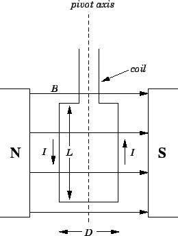
We have talked a lot about potential differences, currents, and resistances, but we have not talked much about how these quantities can be measured. Let us now investigate this topic.Broadly speaking, only electric currents can be measured directly. Potential differences and resistances are usually inferred from measurements of electric currents. The most accurate method of measuring an electric current is by using a device called a galvanometer.A galvanometer consists of a rectangular conducting coil which is free to pivot vertically in an approximately uniform horizontal magnetic field
| (183) |
where
The coil in a galvanometer is usually suspended from a torsion wire. The wire exerts a restoring torque on the coil which tries to twist it back to its original position. The strength of this restoring torque is directly proportional to the angle of twist
There is, of course, a practical limit to how large the angle of twist
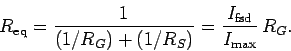
What we do is to connect a shunt resistor in parallel with the galvanometer, so that most of the current flows through the resistor, and only a small fraction of the current flows through the galvanometer itself. Let the resistance of the galvanometer be
| (184) |
which reduces to
| (185) |
Using this formula, we can always choose an appropriate shunt resistor to allow a galvanometer to measure any current, no matter how large. For instance, if the full-scale-deflection current is
| (186) |
Most galvanometers are equipped with a dial which allows us to choose between various alternative ranges of currents which the device can measure: e.g., 0-
 | (187) |
Clearly, if the full-scale-deflection current
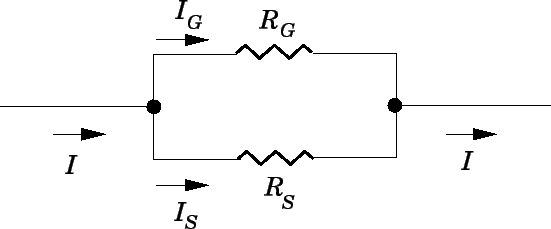
A galvanometer can be used to measure potential difference as well as current (although, in the former case, it is really measuring current). In order to measure the potential difference
| (188) |
which yields
| (189) |
Using this formula, we can always choose an appropriate shunt resistor to allow a galvanometer to measure any voltage, no matter how large. For instance, if the full-scale-deflection current is
| (190) |
Again, there is an advantage in making the full-scale-deflection current of a galvanometer used as a voltmeter small, because, when it is properly set up, the galvanometer never draws more current from the circuit than its full-scale-deflection current. If this current is small then the galvanometer can measure potential differences in a circuit without significantly perturbing the currents flowing around that circuit.
__________________________________________________________________________________

Electronics is the branch of science and technology that deals with electrical circuits involving active electrical components such as vacuum tubes, transistors, diodes and integrated circuits. The nonlinear behaviour of these components and their ability to control electron flows makes amplification of weak signals possible, and is usually applied to information and signal processing. Electronics is distinct from electrical and electro-mechanical science and technology, which deals with the generation, distribution, switching, storage and conversion of electrical energy to and from other energy forms using wires, motors, generators, batteries, switches, relays, transformers, resistors and other passive components. This distinction started around 1906 with the invention by Lee De Forest of the triode, which made electrical amplification of weak radio signals and audio signals possible with a non-mechanical device. Until 1950 this field was called "radio technology" because its principal application was the design and theory of radio transmitters, receivers and vacuum tubes.
Today, most electronic devices use semiconductor components to perform electron control. The study of semiconductor devices and related technology is considered a branch of solid state physics, whereas the design and construction of electronic circuits to solve practical problems come under electronics engineering. This article focuses on engineering aspects of electronics.
Millman's Theorem
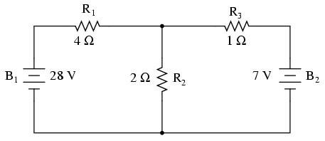
In Millman's Theorem, the circuit is re-drawn as a parallel network of branches, each branch containing a resistor or series battery/resistor combination. Millman's Theorem is applicable only to those circuits which can be re-drawn accordingly. Here again is our example circuit used for the last two analysis methods:
And here is that same circuit, re-drawn for the sake of applying Millman's Theorem:

By considering the supply voltage within each branch and the resistance within each branch, Millman's Theorem will tell us the voltage across all branches. Please note that I've labeled the battery in the rightmost branch as “B3” to clearly denote it as being in the third branch, even though there is no “B2” in the circuit!
Millman's Theorem is nothing more than a long equation, applied to any circuit drawn as a set of parallel-connected branches, each branch with its own voltage source and series resistance:

Substituting actual voltage and resistance figures from our example circuit for the variable terms of this equation, we get the following expression:
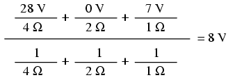
The final answer of 8 volts is the voltage seen across all parallel branches, like this:
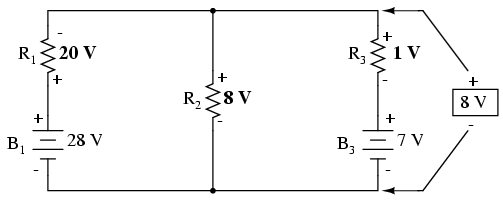
The polarity of all voltages in Millman's Theorem are referenced to the same point. In the example circuit above, I used the bottom wire of the parallel circuit as my reference point, and so the voltages within each branch (28 for the R1 branch, 0 for the R2 branch, and 7 for the R3 branch) were inserted into the equation as positive numbers. Likewise, when the answer came out to 8 volts (positive), this meant that the top wire of the circuit was positive with respect to the bottom wire (the original point of reference). If both batteries had been connected backwards (negative ends up and positive ends down), the voltage for branch 1 would have been entered into the equation as a -28 volts, the voltage for branch 3 as -7 volts, and the resulting answer of -8 volts would have told us that the top wire was negative with respect to the bottom wire (our initial point of reference).
To solve for resistor voltage drops, the Millman voltage (across the parallel network) must be compared against the voltage source within each branch, using the principle of voltages adding in series to determine the magnitude and polarity of voltage across each resistor:

To solve for branch currents, each resistor voltage drop can be divided by its respective resistance (I=E/R):

The direction of current through each resistor is determined by the polarity across each resistor, not by the polarity across each battery, as current can be forced backwards through a battery, as is the case with B3 in the example circuit. This is important to keep in mind, since Millman's Theorem doesn't provide as direct an indication of “wrong” current direction as does the Branch Current or Mesh Current methods. You must pay close attention to the polarities of resistor voltage drops as given by Kirchhoff's Voltage Law, determining direction of currents from that.

Millman's Theorem is very convenient for determining the voltage across a set of parallel branches, where there are enough voltage sources present to preclude solution via regular series-parallel reduction method. It also is easy in the sense that it doesn't require the use of simultaneous equations. However, it is limited in that it only applied to circuits which can be re-drawn to fit this form. It cannot be used, for example, to solve an unbalanced bridge circuit. And, even in cases where Millman's Theorem can be applied, the solution of individual resistor voltage drops can be a bit daunting to some, the Millman's Theorem equation only providing a single figure for branch voltage.
As you will see, each network analysis method has its own advantages and disadvantages. Each method is a tool, and there is no tool that is perfect for all jobs. The skilled technician, however, carries these methods in his or her mind like a mechanic carries a set of tools in his or her tool box. The more tools you have equipped yourself with, the better prepared you will be for any eventuality.
Goals Of This Lesson
Thevinin Theorem
Why Use Thevenin Equivalent Circuits?
Whenever you need to predict how something is going to behave you don't need to analyze things down to the lowest possible level. For example, when current flows in a resistor, you don't need to know what happens to every atom in the resistor. That ability to describe what happens to a large number of atoms in the resistor by using a macromodel for the resistor is convenient. Electrical engineers often think at different levels of complexity.
- When analyzing/describing an amplifier circuit or a digital logic circuit the designer uses a macromodel for the resistors, transistors, capacitors and other components and doesn't worry about what happens inside those components.
- When analyzing/describing a logic chip the designer uses a macromodel for the gates in the logic circuits, and doesn't worry about the transistors, etc. that comprise the innards of the logic circuits.
- When analyzing/describing a computer, the designer uses a macromodel for the logic chips and doesn't worry about the gates inside the chips.
Goals Of This Lesson
What do you want to know about Thevenin and Norton equivalent circuits.
- Given a source - not an ideal source,
- Be able to determine the Thevenin and Norton equivalent circuits for simple circuits,
- Be able to predict behavior under load for a non-ideal source.
- Computer networks composed of computers,
- Computers composed of various kinds of integrated circuit chips, etc.,
- Integrated circuit chips composed of gates and other logic circuits,
- Logic circuits composed of transistors, resistors and other electronic components,
- Transistors composed of atoms of semiconductor material,
- Atoms composed of protons, electrons, etc.,
- Protons composed of quarks.
When you want to use different components you often need to use macromodels of the components you use. You do that because you don't always need to have totally detailed knowledge of what goes on inside the component.
Thevenin Equivalent Circuits - or TECs - are macromodels that are used to model electrical sources. Those sources are as diverse as batteries, stereo amplifiers and microwave transmitters. In this lesson we will develop TEC models of sources and learn how to use them in larger circuits.
What Is A Thevenin Equivalent Circuit?
The Thevenin Equivalent Circuit is an electrical model composed of two components shown below.

- An ideal voltage source, Vo.
- A resistor, Ro.
We can write equations that describe the behavior of the TEC when it interacts with other components. First, let us define some variables. If we have a load attached to the terminals some load current will flow. We'll define a load current and a terminal voltage for the TEC as shown below.


Finding A Thevenin Equivalent Circuit
The TEC is a useful way of reducing complexity. If you have a complex circuit interacting with other circuits you don't want to look at all of the details of what is taking place inside the complex circuit - at least you don't often want that.
To illustrate some of the power of the TEC we'll get the TEC for a voltage divider.

The voltage divider isn't a very complex circuit, but it is more complex than the TEC. It can be represented with a TEC, and wherever you find a voltage divider you can replace it with the equivalent TEC. We need to establish values and/or formulas for two items in the voltage divider. Basically, we need two of the following:
- Open Circuit Voltage
- Internal Resistance
- Short Circuit Current.


Next, focus on theShort Circuit Current. Short circuit current, Iois the current that would flow if the output of the circuit is short circuited. We can imagine shorting the Voltage Divider and shorting the TEC. Wires that short them are shown below and the short circuit current, Isc, is indicated.

For the TEC you should be able to see quickly that the short circuit current is just
Vo / Ro . For the voltage divider it's not any more difficult. There the short circuit current is just Vs / Rb. We can use both of these observations to compute the internal resistance of the voltage divider TEC.

Calculate the Short Circuit Current.
Combining we have
Continuing, we find:
= RaRb /( Rb + Ra)
So, we have the internal resistance, and it looks like the parallel formula. (But it really isn't!)
At this point you can compute both the open circuit voltge and the internal resistance for the voltage divider, so you have a TEC for the voltage divider. You can use that TEC any place you find the voltage divider. It doesn't matter where you find the voltage divider, you can replace it with its TEC, just like you can replace two parallel resistors by their parallel equivalent.
Norton Theorem
Norton Equivalent Circuits
In electrical engineering there is a recurring duality. Voltage and current are duals, and where we find one variable appearing in an expression or a theorem, we usually find the other appearing in a dual expression or theorem. The dual of the Thevenin equivalent model is the Norton equivalent model, a sample of which is given in the figure below.
The relation between terminal voltage and load current for this circuit is interesting because it is indistinguishable from that of the Thevenin Circuit, and the two are electrically equivalent. Write KirchHoff's Current Law for the Norton circuit with a load attached. The result is:
 Vterminal/Ro + Iload = Io
So, we find:
If we identify RoIo with the Vo that appears in the Thevenin model, this is, as claimed, equivalent to the Thevenin model.
Note the following relations between the Thevenin and Norton equivalents.
- The internal resistance, Ro, is the same in both the Thevenin and Norton circuits.
- Vo = RoIo, where
- Vo = Open Circuit Voltage in the Thevenin model, and,
- Io is the short circuit current in the Norton model.
- Both circuits satisfy:
- Vterminal = RoIo - RoIload = Vo - RoIloa
The Maximum Power Theorem
Whenever we have a source of electrical energy we might pose the question of what circumstances produce maximum load power.
- Teenagers solve a closely related problem whenever they are able to determine the speaker connections that produce the maximum amount of noise from a stereo system.
- Engineers processing radar signals solve the same problem when they extract the maximum power from a low power signal received through an antenna.
Consider a load connected to a source, and consider that the source is well represented by a Thevenin equivalent model. Then the situation is the one shown in the figure below.

The question we want to answer is:
- What load will dissipate the maximum amount of power when connected to the given source?
- First calculate the voltage across the load resistor, calling that voltage Vload.
- Vload = Vo Rload/(Ro+ Rload)
- Then the power dissipated in Rload is:
- (Vload)2 / Rload
- = (Vo)2 Rload/(Ro+ Rload)2
The maximum power for positive load resistance occurs when:
When the load resistance is equal to the internal resistance of the source, the load voltage is exactly half of the open circuit voltage, so the maximum power delivered to the load is:
Whenever a load resistance is equal to the internal resistance of a source, the two (source and resistance) are said to be matched.
Some Reflections
Above we have derived the maximum power theorem as it is usually presented. However, it gives the impression that maximum power is delivered only when a resistive load equal to the internal impedance is attached. That is not the case!
- Maximum power is delivered to a load when it drops the terminal voltage to half the open circuit voltage and the load current is half the short circuit current.
- However, that is not quite what we proved, so let us look at a more general situation.
- You have a source with a relationship between terminal voltage and load current as shown in the graph below.

The load power is given by:
Now, differentiate with respect to Iload.
Now solve for the load current that maximizes load power, and we get:
That's half the short circuit current, and if you put that value back into the equation for terminal voltage, the terminal voltage at max power is half of the open circuit voltage.
To give another perspective, consider that the power to the load - VloadIload- can be thought of as the area of a rectangle at a point on the load curve for the source. At any point on the plot of terminal voltage against load current, the product of the terminal voltage and the load current is the power delivered. That's also the area of a rectangle with a height equal to the terminal voltage and a width equal to the load current. Thus, we can look at the rectangle under the load curve for a series of points and the point with the rectangle with the largest area is the point which delivers the most power to the load.
- Click the double arrow green button below to see how that rectangle area varies as the point moves along the load line.
- Click the single arrow green button to step the action one step.
- Click the single arrow green button pointing left to back up the action once it is started.
- Estimate the point at which the area of the rectangle is largest - remembering that the area of the triangle is the power delivered to the load.
- Can you see that there is a max?

To try to determine the maximum power that can be extracted from this solar cell is more difficult than when the load curve is a straight line. However, some of the ideas we have used so far may also be used here. For example, the power supplied by this source may still be viewed as the area of a rectangle at a point on the curve. You can check that below.
Here's the solar cell load curve again. Here you can click to see three different operatin point, and you can determine which operating point provides the most load power. Remember, the power supplied will be the product of load voltage and load current, so it is the area under the rectangle that shows. Click each button to see a point on the load line and a rectangle whose area is the power supplied when the solar cell at that point.
Here are a few points to note
- Clearly, the max power point occurs near the rounded corner at the top right.
- When the max power is delivered, the load voltage is well above half of the open circuit voltage, and the current is nearly the short circuit current.Using TECs In Circuit Analysis One common circuit is a voltage divider. Here is a voltage divider.

- A voltage divider is a linear circuit,
- Therefore, a voltage divider has a Thevenin Equivalent Circuit.
- The unresolved question is how to determine the TEC.
- In the process we can learn how to use Thevenin and Norton equivalents to simplify circuits, including source conversions.
Now, any time we have a Thevenin equivalent circuit we can replace it with a Norton equivalent. That's what we will do below. Recall:
- The short circuit current = Open circuit voltage/Internal resistance.
- The internal resistance is the same for the Thevenin and the Norton circuits.
You can click the button to initate the transformation from a Thevenin Equivalent to a Norton Equivalent. (And you can click it again to reset back to a TEC.) Now, if your expert genes are still working you will recognize a combination in the Norton circuit.
Now, you can combine the two resistors in the combination. If you do that, you should get the circuit below.
 Now, the two resistors, Raand Rb, are in parallel, and they can be combined to give the circuit below.
- This is the Norton equivalent circuit for the voltage divider.
- If you want the Thevenin equivalent circuit, you can convert the Norton equivalent to a TEC by computing the open circuit voltage.
- The open circuit voltage is given by:
- Vo = (Vin/Ra) (RaRb/(Ra + Rb))
- The result is the TEC shown below.
 Notice the equivalent circuit has the following properties.
- The open circuit voltage is the voltage we get from the voltage divider formula.
- The internal resistance has a formula for a parallel resistance even though the two resistors would appear to be in series in the original voltage divider.
What If You Can't Calculate The TEC? If you can't calculate the TEC, there is always the possibility of measuring the TEC. To measure the TEC you can often measure the open circuit voltage pretty easily. Measuring the internal resistance is a different problem. To do that you almost certainly have to attach a load to the source to cause the terminal voltage to drop. That might be a problem with a source like the plug on the wall, for example. You might not want to draw enough current from the wall plug to drop the voltage enought to measure the difference. Spots in the wiring inside the wall could get hot - possibly enough to start a fire.
What If You Need To Know About Things Inside The Source?
Sometimes you need to know about variables inside a source. For example, in the voltage divider, you might want to know how much power is consumed in the resistors in the voltage divider. You can't tell anything about that from the TEC. You have to go back to the actual circuit in that case.
The TEC can't do everything. What it does is enable you to use a simple model to predict how a real source - no matter how complex - interacts with the rest of the world. But it doesn't tell you about what goes on inside the source itself!